Commercial highlights
- released in late 2018
- 50+ projects to date for 25+ different clients
- more than 18,000 sqkm and 230+ wells
Client value
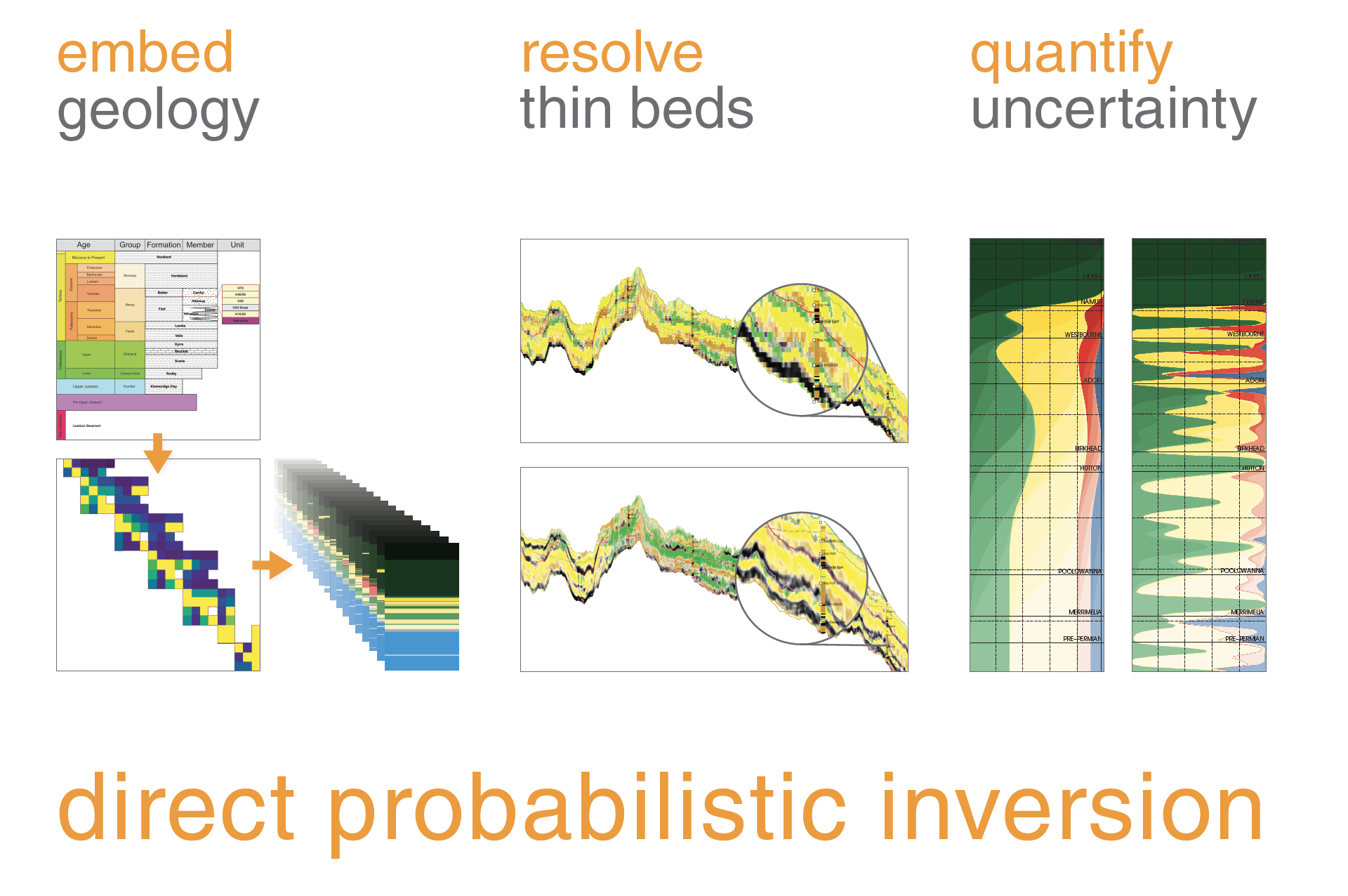
- robust quantification of uncertainty
- thin bed resolution (below seismic tuning thickness)
- differentiates between facies that overlap in elastic space
Technical highlights
- Bayesian inference technique
- demonstrated in land and offshore settings and on 2D, 3D, 4D and PPPS data
- probabilistic prior consists of geological observations and rock physics models
- can incorporate any reflectivity model
- can incorporate VTI anisotropy
- numerous published technical papers and case studies

DPI videos
Direct facies inversion from seismic
DPI - case studies
DPI - a deep dive into the algorithm
Anisotropic DPI
DPI publications
Anisotropic Direct Probabilistic Inversion for unconventional tight reservoirs
Depth trends in facies classification using Direct Probabilistic Inversion
Inversion of thin-bedded multi-lithology settings
Direct Probabilistic Inversion for facies using the Zoeppritz reflectivity model
Facies classification and surface interpretation using Direct Probabilistic Inversion of AVO data
Direct Probabilistic Inversion of seismic AVO data for reservoir characterization
Combined stratal geometry and seismic inversion characterisation of sand distribution, Cambo
Seismic inversion of dual azimuth broadband seismic data
Reservoir characterisation in the presence of thin beds and elastically ambiguous facies.
Exploring noise models in approximate Bayesian inversion for facies
Reservoir characterisation in the presence of thin beds and elastically ambiguous facies
Reservoir characterisation by Direct Probabilistic Inversion
The who's who of DPI

Ask Frode Jakobsen
Founder
Principal developer DPI

Bill Goodway
Scientific Advisor
Custodian DPI geophysics

Henrik Juhl Hansen
Founder
Principal developer DPI

Raul Cova
Lead Geophysicist
Developer anisotropic DPI
Direct Probabilistic Inversion - A technical description
Traditional geostatistical inversions rely on the expensive and slow Hastings Metropolis Markov chain Monte Carlo type algorithms (HMMcMC). The variant HMMcMC approaches deployed can suffer from a number of drawbacks:
- Computationally expensive
- Open questions on independence of realisations
- Open questions on convergence
- Limited sampling of the unknown solution space hence difficult to comprehend uncertainty
Qeye proposes a unique approach to invert for either seismic facies or reservoir properties directly. The method is a Bayesian inference type approach– this is a machine learning technique well described in the machine learning literature which Qeye is using in the oil and gas arena.
A statistical prior model is constructed that is based on the available well database and that describes the distribution of unit thicknesses and the rules for transition between one facies and the next (imposed stratigraphic ordering and gravitational fluid ordering). The approach is extremely flexible and allows for transitions from each facies to any other facies within a probabilistic framework.
The conditioned seismic amplitudes and associated wavelets are then input to an inversion directly for the facies (or properties). This approach has a large number of advantages over current methods, either the so called “facies aware” or “joint facies” inversions or Hastings-Metropolis style geostatistical inversions.
- The inversion is no longer pointwise but spatially aware– it is more stable and produces results from a physically and geologically plausible solution space explicitly defined by the geological depositional model.
- The non-uniqueness of the inversion is handled explicitly and in a robust manner. Physically plausible property distributions away from the most likely result are available coupled with a likelihood. This information can be used in scenario planning in the same way that the most likely result can be used.
- There is no biasing of the solution with spatial information from a structural prior model. The inversion is agnostic even of interpreted surfaces.
- The results are more data driven and hence less biased by preconception.
The mathematical impact of this is that the solution space is broad yet constrained only to those solutions that are plausible – in contrast MCMC methods have solution spaces that are implausibly large. What this means for the end user is that geologically or petrophysically impossible (or highly unlikely) solutions are removed (or downweighted) and will not feature with high posterior probabilities in the outcomes.
Simple examples of these weaknesses manifest in other methods results could be:
- water sands predicted directly above oil sands
- package responses delivered at seismic resolution instead of interbedded facies below seismic resolution
- older units predicted above younger units
In the direct inversion proposed by Qeye the input data are expressed as probability density functions. The prior statement is extremely smooth and consists of thickness distributions for the facies and transition rules for facies to be placed in neighbouring cells (as a simple example the vertical transition from water sand downwards to oil sand can be set to 0%). Both the thickness distributions and the transition rules can draw from wells in a wider area than the survey and can be informed by geological interpretation of the area.
The seismic reflections are then directly inverted for the facies within the constraints of the prior statements. This means that, because the prior statements contain beds below tuning thickness these will be considered by the inversion as plausible solutions, however implausible transitions (such as an older shale over a younger shale) are rejected. This also means that elastically very similar (or identical) facies that are separated stratigraphically are discriminated in the inversion results.
This approach allows a robust handling of uncertainty and non-uniqueness and avoids making pointwise rather than local or global assumptions.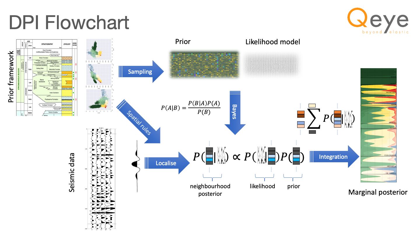
The Direct Probabilistic Inversion Scheme (Jakobsen et. al, SEG 2019). The novel formulation of the prior framework and the localisation of the problem enables computationally efficient estimates of the posterior to be derived.
The workflow can be described thus:
Generate facies constellation
- Identify N facies/units
- For each facies combination (n,m) define P1(n,m) – the probability that m in below n
- For each facies n define P2(n) – the probability distribution for that facies thickness
- Use P1 and P2 to frame the subsurface as a Markov process
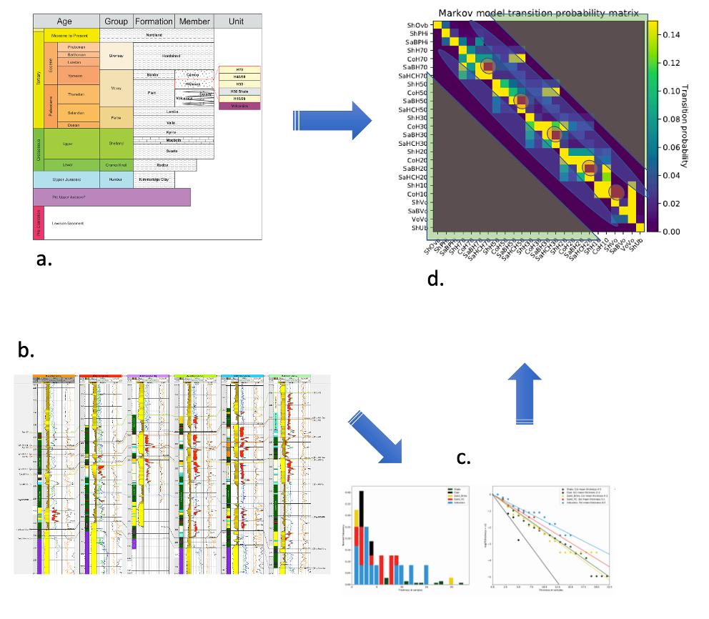
(a) A stratigraphic framework (together with other interpreting information and well logs) defines a list of units/facies and the transition probabilities. [Offset] wells logs define the unit thickness distributions; these are typically fitted to a log-normal linear distribution (c). Finally (d) this information is combined into a first-order Markov process that describes the sub-surface. Note that: (i) extremely low energy in the process away from the lead diagonal (green triangles) enforces stratigraphic ordering; (ii) energy levels off the lead diagonals accounts for faulting, unconformities, geological inversion etc. as required by the data and the interpretation (blue ellipses), and; (iii) fluid gravitation ordering is enforced by zero transition probabilities on the leading diagonal (and elsewhere) (orange circles).
Statistical rock physics
For each facies/unit n define a statistical rock physics model for AI, Vp/Vs, ρ. The rock physics models incorporate VTI anisotropy, property correlation length, and co-variances between the properties.
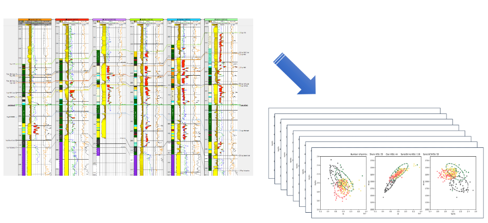
From the [offset] [fluid/porosity/mineral substituted] well log data a statistical rock physics model is derived for every unit/facies to be inverted for.
Likelihood modelling
Sample the functions from the first two steps to generate a large number M of permitted unit configurations (prior) and a large number M’ of elastic representations of each permitted configuration (likelihood function) sampling for all facies configurations (n1, n2, … nx, …. nN).
As this process is linear and 1D it can be highly parallelised. The process is also relatively low compute cost. These two factors enable extremely dense and wide sampling of the solution space.
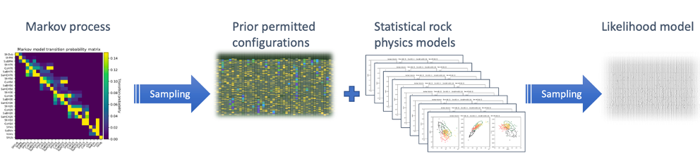
Process flow diagram from 1st Order Markov process to Likelihood model.
Bayesian Inversion
Estimate the full marginal posterior facies distribution by applying Bayes theorem to the seismic for each configuration (n1, n2, … nx, …. nN). This step is also 1D and so can be highly parallelised.
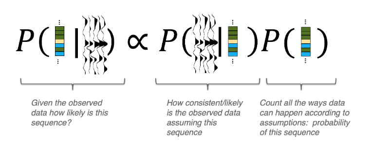
Bayesian Inference as applied in DPI. The left-hand side is the unknown and the right-hand side is how closely the seismic represents the associated likelihood models multiplied by how many times this configuration occurs in the prior configuration sampling.
Integration
The final step is to gather all of the neighbourhood posteriors (see Figure 14) for each sample in the volume by common central facies and sum, normalising the sum of all these sums such that the total probability at each same is unity.
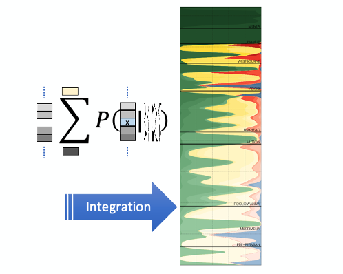
For every possible central facies (x) sum the neighbourhood posterior across all possible facies configurations. Repeat for every sample of every trace.
In the example shown below a prior statement has been constructed using a number of wells in the area and the interpretations of the field geologists.
- ten shale units are identified (in green dark to light is young to old).
- eight sands are identified each sand can be
- brine (in yellow dark to light is young to old) Or
- hydrocarbon charged (in red dark to light is young to old)
- four cemented sand facies are also identified (in blue dark to light is young to old).
In this example a total of 30 discrete facies – each with their own properties, thickness distributions and transition rules form the prior statement.
The figure below illustrates the power of the direct inversion method. The petrophysical logs at the well are shown on the left. The next panel is the facies log from the well. The third panel is a visualisation of the prior statement for the project. Important to note is that the prior statement is exceptionally smooth and broad, it places very little constraint on the facies. This visualisation captures some of the vertical ordering but does not show the full dimensionality of all the allowed and forbidden transitions.
The final panel shows the inverted results. Note how the intra Namur shales or the exceptionally thin Adori hydrocarbon and cemented sand legs are identified despite being at the limit of resolution in the seismic. Also note that every same in the volume is now a probability function of each of the 30 facies (with most of these a posteriori probabilities being very close to zero).
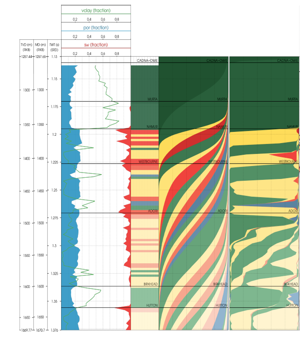
A direct facies inversion result from a recent project. The panels left to right are the petrophysics and facies interpretations at the well location. The prior facies distributions and the posterior facies distributions. Note how, using this direct facies method, exceptionally thin beds can be resolved with reasonable confidence.
In this next example a comparison is made between a traditional lithoclass workflow and the DPI workflow. Note the:
- improved resolution
- characterisation of extremely thin coal facies – one or two samples at 1ms sample rate
- improved fluid discrimination
- excellent well ties (note that all wells are “blind” – only their statistics are used in the inversion framework
In this example DPI outperforms lithology classification by 30% (51% overall accuracy vs well logs for DPI compared to 39% for lithoclass). It is worth noting that the DPI statistic of 51% represents an approximation to the average results quality across the volume whereas the lithoclass 39% is approximately the best result anywhere in the volume, this is because the lithology classification PDFs are derived from the well data at the well locations, whereas the DPI uses global statistics.
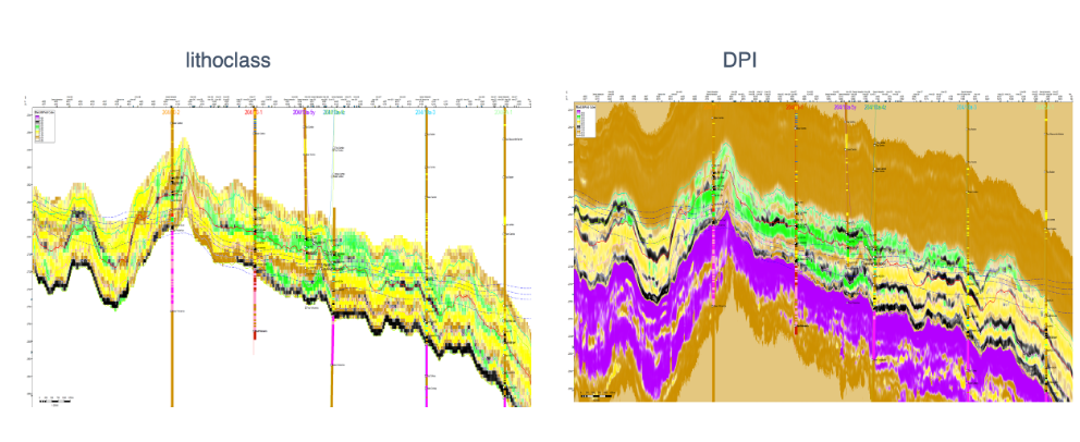
Comparison of a traditional lithoclass workflow vs DP. This example from Cambo field West of Shetlands, UK, and is courtesy of Siccar Point (after Poore et. al. 2020). Note the correctly place fluid contact, the thin bed resolution (coals), the correct NTG vs the lithoclass over prediction of sand and the excellent well ties. This and other detailed case studies are available on request.